
01: Foundational Explanations & Capabilities
-
Beyond A∗: Better Planning with Transformers via Search Dynamics Bootstrapping
Orca: Progressive Learning from Complex Explanation Traces of GPT-4
Personality Traits in Large Language Models (Jul 2023, added 7/14/23)
LLMZip: Lossless Text Compression using Large Language Models (Jun 2023, added 6/24/23)
The Simplest Description Of The Classical Transformer Architecture (Jun 2023)
An Overview On Language Models: Recent Developments And Outlook (Mar 2023)
Harnessing the Power of LLMs in Practice: A Survey on ChatGPT and Beyond (Apr 2023, added 5/7/23)
What Algorithms Can Transformers Learn? A Study In Length Generalization
Large Language Models Can Learn Rules, pt I
(Oct 2023, link)
This is a cool paper that introduces a very specific trick to teach LLMs how to “learn” large, formal rule bases. A rule base here is a long list of statements that the LLM needs to piece together to solve some particular question. (Famous example: Rule 1- Socrates is a man, Rule 2- All men are mortal, Deduction- Therefore, Socrates is mortal.) First, here is a simple example for such a rule base: adding numbers in base-9 (not base-10: meaning, 6 + 4 = 11, because 11 = 9^1 + 9^0). We give the LLM the rules that are listed in the Rule Library, consisting of both positive and negative rules. (See the Rule Library simply listed under “Knowledge:” in the prompt.)
Notice in the chart above that their algorithm has two stages: induction and deduction. In the induction stage, they use GPT-4 to first generate the rule base. They do that by giving lots of samples, verifying whether GPT-4 answers correctly by chain-of-thought, and then adding the sub-rules that GPT-4 identified as necessary to solve the problem to the rule base. In the deduction stage, they then simply put all those generated rules into the prompt for in-context learning, and let the LLM do the problem solving.
What they find is that GPT-4 is pretty bad at incorporating rule bases! In 0-shot chain-of-thought prompting, for 4-digit base-9 addition, it only gets 23.1% of the tests right. In 5-shot chain-of-thought, that goes up to 42.3% (i.e., giving 5 examples in the prompt). (LtM is the least-to-most prompting methodology presented in another paper - yet another prompting technique.)
But now their trick comes into play: instead of just listing all these base-9 rules, surround them with a kind of mark-up language, so that GPT-4 has an easier time retrieving the right rule. This is done with a simple form of “XML tagging”: instead of just listing 0 + 0 = 0 and 3 + 0 = 3, they add two XML tags in front of each rule. One is the first operand, the second is the second operand. So 3 + 0 = 3 becomes <3><0>3 + 0 = 3.</0>...<3><9>3 + 9 = 13.</9>...</3>. This simple “categorization” makes it easier for GPT-4 to spot the rule it needs, at inference time. This is a really good trick that should work elsewhere, when trying to put content into the prompt.
The table above shows that this lifts 5-shot chain-of-thought accuracy from 42.3% to 65.4%.
How many samples do you need to give in the induction stage to construct a good rule base? You get better performance by adding more samples, see the chart below.
How many rules does the LLM discover in the induction stage? First, note that there is an actual computable number of rules that you can derive from a particular number of samples - namely, all the combinations of digits you’ve seen so far in your, say, base-9 addition samples (like, 6 + 3 = 9 gives you exactly that one rule, but multi-digit examples give you several rules per example). The chart below shows that maximum number of derivable rules by number of samples, and the percent of those that GPT-4 “discovers” by itself, in the induction stage. Interesting (and not clear why the difference).
Large Language Models can Learn Rules, pt II
Nov 2023, here
This paper has a really clever idea on how to load a large number of rules in a rule base into a prompt, while not overloading the LLM: by tagging rules with XML tags in a hierarchy.
Here is the actual challenge the paper is trying to solve: in an induction stage, we derive a bunch of rules for a rule base we’d like to build (left). In the deduction stage, we ask the LLM to apply those rules (right). The example below is for addition in base-9: we generate a large rule library of how to do those additions by running a whole bunch of examples. (For example: 6 + 4 != 10 because this is base-9, so 6 + 4 = 11.)

Then we simply pre-pend all of those rules to the prompt in the deduction stage! So the LLM can use those rules to reason. Here is the problem: if you pre-pend that many rules, the LLM usually gets confused and fails.
Now the paper’s clever idea: a) turn the rules into a hierarchy and b) tag the rules with XML tags so it’s easy to navigate the hierarchy. This should make it easy for the LLM to first find the right level in the hierarchy, and then look up the actual rule. Here, the hierarchy is split into two levels: in a sum 3 + 1 = 4, the first hierarchy is the first operand, and the second level is the second operand, like in the screenshot below. So first you list all the 0 + x, then all the 1 + x, etc. XML tag <3>...</3> lists all the 3 + x. And the tag <3>...<4>3 + 4 = 7</4> ... </3> has the rule we want.

Turns out this works very well!
Grandmaster-Level Chess Without Search
(Feb 2024, link )
This is another example for the power of a transformer to implement a powerful algorithm, without our really knowing how it does that: here, a transformer (not pretrained with language, but pure) generalizes to being a powerful chess engine.
The basic algorithm is extremely simple:
Take a collection of 10 million chess games
Extract all board states (all figure positions) from these games. Encode a board state in a simple text-based prompt.
Run each board state through the world’s best chess engine Stockfish 16, to generate a “state value” for each board state. The state value is the win probability for this exact board state, based on what Stockfish thinks.
Finally, extract “action values” for each board state in our dataset: for each legal action in a particular board state (i.e., all moves we can legally do with any of the remaining figures on the board), simply get the next board state (what does the board look like after taking this one action), and ask Stockfish what the win probability is for that new board state.
(Separately, the paper also collects 10K particularly challenging puzzle board positions from its original chess game source, which come with a correct sequence of chess moves to solve the puzzle.)
That’s it, extremely simple! We just give chess games to the transformer, and we give it the ground truth win probability. If we do that with various transformer sizes, we get the following performance. Quite amazingly, the transformer becomes a better chess player than AlphaZero, and compares quite well to Stockfish 16.
Here is a very cool table that looks at some of the design decisions of the paper, and how they impact the outcome. First, they test three different ways to “play chess”:
AV (action value) means giving the transformer the concatenation of board state and a particular action and letting it predict the board state win probability, so we can simply pick the action that maximizes that after trying all legal actions;
SV (state value) gives the transformer just a board state and predicts that board state win probability, and we use it by manually generating all board states from plugging in all legal actions and getting the next board state and picking the one that best minimizes our opponent’s win probability;
BC (behavioral cloning) gives the transformer just a board state and predicts the action with the highest win probability from the current board state. So unlike the other two choices, this one doesn’t just produce one win probability, but a win probability for all legal actions.
It looks like the choice of “predictor-target” makes a huge difference, but the paper realizes that this is just because the training sets for those are somewhat different. If you correct for that, the choice actually makes almost no difference, which is interesting! Trying to engineer a better transformer by picking a smarter optimization target makes no difference.
The other one that is very interesting here is “network depth”: that is the number of hidden layers of the transformer. The paper does something very clever here in keeping the transformer’s parameter (weight) count always the same - so when it reduces the number of layers, it increases 1) the layer width (weights per layer) and 2) the embedding dimensions. It is remarkable that network depth only matters up to a certain point - it doesn’t improve things beyond 8 layers.
Beyond A∗: Better Planning with Transformers via Search Dynamics Bootstrapping
(Feb 2024, link)
Very interesting paper: it shows that we can take the “navigation trace” output from running the well-known A* search algorithm on mazes, take that trace, and train a transformer on it. The transformer seems to then generalize to be able to run A* all by itself, on unknown mazes.
First, here is an example for navigating a maze: the prompt sets up the maze (the numbers are coordinates, and we specify start, end and wall locations), and the response lists the step-by-step coordinates. So, we want a transformer to which we can give that prompt, and it produces that response.
Now, here is how A* would solve this. The exact details of A* really aren’t that important (it’s a clever search algorithm that uses various sets and costs to keep track of nodes while exploring a maze and backtracking). But what’s important is that running the algorithm creates a step-by-step trace - including all the A*-internal steps, i.e., not just the resulting navigation itself. (“Close 0 2 c3 c0” is when the A* algorithm keeps track of a node by pushing it onto a set, for example.)
The paper does something seemingly simple: it creates lots of mazes, it then creates lots of A* navigation traces, and then it trains a pure transformer on those traces. In fact, and this will become important later, it creates two outputs: (1) the A* and navigation trace (“search-augmented sequence”), and (2) only the navigation trace without the A* commands (“solution-only sequence”). Note that these are impressively long sequences - the solutions are pretty short (a few dozen steps), but the A* traces are really long (thousands of tokens):
It is surprising how well this works! After training a relatively small transformer, that model is able to navigate mazes optimally. But it’s also very interesting to see the difference between “search-augmented” and “solution-only”: for solution-only, we didn’t teach the transformer anything, we just showed it lots of navigation solutions. And yet, larger transformers are able to even learn from that. But if we give the transformer the A*-augmented traces, it generalizes with much smaller training data.
On the right side, the paper does something else that’s very interesting: there are various ways in which we can randomize the A* algorithm, for example by randomizing the order in which nodes “on the stack” are explored. Those are all still optimal, but they change up the original order. When we use a training set that was created with such a more randomized A* algorithm application, then the transformer generalizes even better for small training data sets. It doesn’t help the solution-only set.
Now we come to a final, pretty awesome discovery: by generating specific training data sets with shorter and more optimal navigation solutions, we can get the transformer to become better at solving mazes. The idea is really simple: first, do exactly what was laid out above, and train a transformer on A* with a training set derived from sample mazes. Then, use that search-augmented transformer (described above), and only pick the shortest paths for particular maze solutions (we can get more than one solution per maze by randomizing A* somewhat, as described above), and that becomes a new training dataset. Use that dataset to fine-tune the original transformer. That is step 1. Then, do that two more times - each time, using the newly created transformer to create shorter and shorter solutions to various mazes, and fine-tune the transformer with that augmented dataset.On the right side, the paper does something else that’s very interesting: there are various ways in which we can randomize the A* algorithm, for example by randomizing the order in which nodes “on the stack” are explored. Those are all still optimal, but they change up the original order. When we use a training set that was created with such a more randomized A* algorithm application, then the transformer generalizes even better for small training data sets. It doesn’t help the solution-only set.
Now we come to a final, pretty awesome discovery: by generating specific training data sets with shorter and more optimal navigation solutions, we can get the transformer to become better at solving mazes. The idea is really simple: first, do exactly what was laid out above, and train a transformer on A* with a training set derived from sample mazes. Then, use that search-augmented transformer (described above), and only pick the shortest paths for particular maze solutions (we can get more than one solution per maze by randomizing A* somewhat, as described above), and that becomes a new training dataset. Use that dataset to fine-tune the original transformer. That is step 1. Then, do that two more times - each time, using the newly created transformer to create shorter and shorter solutions to various mazes, and fine-tune the transformer with that augmented dataset.
What we find in the final step is this: the length of individual solution sequences in the Searchformer (the three-times fine-tuned transformer) skews much shorter. This is an excellent example for a) the transformer generalizing to some kind of A* variant that can solve mazes, and b) getting more optimal through fine-tuning on shorter paths.
Language Models can be Logical Solvers
(Nov 2023, link)
This paper’s basic idea is very similar to that of the Searchformer (“Beyond A*”) paper here: if we want to teach a transformer how to implement a particular algorithm, then we should give it lots of training data that shows the exact step-by-step application of that algorithm - not just the final solution output. In the A* paper, the training data was the turn-by-turn navigation of applying the A* search algorithm to navigating mazes. In this paper, the training data is the step-by-step application of a logical solver (effectively, Prolog), getting applied to predicate logic statements.
The paper starts with a simple idea: we can give an LLM text, and then ask it to map that text into logical statements that are compatible with the solver Prolog. We can then hand those statements over to Prolog, and Prolog will do the actual logic execution for us, and give us the solution. An example is below.
But here is now the idea: we can instead ask Prolog to generate all the intermediate rule application steps that it uses to get the solution. That gives us a trace. See the example below (in colors).
We can then produce lots of those traces. That gives us good training data (entirely text-based). We can use that training data to fine-tune our language model. (Here, we have a big difference to the A* paper: that paper trained a pure transformer from the ground up, whereas this paper fine-tunes a language model. Interesting that both work!)
This works really quite well: on two benchmarks, their fine-tuned CodeLlama-13b performs better than all other LLMs.
One more interesting observation: when prompting with few-shot examples, open-source LMs exhibit notably poor deductive reasoning capabilities, with their outputs closed to random answering. This once again demonstrates that it is considerably difficult for many LLMs to solve logical reasoning tasks. That is quite staggering!
But, it is equally staggering that a relatively simple fine-tuning process on this kind of “algorithm exhaust data” then enables those same LLMs to get really good at this. Is this just a weird example of overfitting and memorization, or is there more (generalization) going on?
A final observation that is also stunning: the paper looks at the impact of simple notation. In the table below, it fine-tunes based on training data that makes certain changes to its notation. For example, it removes the “unbind” statements from the Prolog trace (that’s when Prolog overwrites a variable with another value). That doesn’t turn out to make much of a difference. But: “w/ NL representation” has a huge impact. That just means that the symbolic language (SL) representation “Green(’Charlie’, True))” is replaced by its original natural language (NL) “Charlie is green”. Big insight: notation matters.
Orca: Progressive Learning from Complex Explanation Traces of GPT-4
(Jun 2023, link)
Lots of papers have used GPT-4 output to do instruction-tuning on smaller open-source LLMs: you get great training data out of GPT-4, and you can use that to fine-tune. This paper takes this a step further: instead of just generation <query, response> pairs, also generate lots of chain-of-thought data. It turns out that improves the quality of the fine-tuned LLM. For example, on BigBench-Hard, this improves significantly on the already instruction-tuned LLM Vicuna-13B:

Here is how they do it: ask GPT-4 for high-quality instruction traces. Here is an interesting thing: they don’t just use one system prompt, they use several different ones - “think step-by-step and justify your steps”, or “provide a detailed answer so users don’t need to search outside to understand the answer”. That variety might actually help. They use a total of 16 system messages. Unfortunately, they don’t test whether using fewer or more of these leads to any differences in quality of output.

Personality Traits in Large Language Models (Jul 2023, added 7/14/23)
(link)
Good foundational insight: you can prompt LLMs into adopting a “personality”, and it will produce output that is consistent with the associated personality traits. To do that, the paper does the following:
Pick the right personality tests. For example, the Big Five Inventory, BFI: identifies five personality trait dimensions - extraversion (EXT), agreeableness (AGR), conscientiousness (CON), neuroticism (NEU), and openness to experience (OPE).
Ensure structural validity of a test. Is the test reliable across multiple measurements (i.e., its items)? In other words, do responses to the test’s items form consistent patterns? Do the test’s items reflect the variance of one underlying factor or construct?
Ensure external validity of a test. Are the test scores practically meaningful, outside (external to) the test context itself?
Here is the flowchart the paper follows to administer personality tests to LLMS:
Here is how the LLM gets prompted for each question in a personality test: each question gets prepended with short biographical statements sampled from a repository. Then the question is administered.
After generating these biographical statements and administering the chosen personality test (the paper uses a test called IPIP-NEO), the paper calculates structural and external validity.
Structural validity: This analyzes whether the model’s personality is self-consistent. This is calculated by simply calculating various formal metrics, like “Cronbach’s Alpha” - the idea for all of these is that psychologists that built the IPIP-NEO test looked at which questions should correlate with each other, and you can simply calculate whether the model’s answers are consistent in that way.
External validity: This analyzes whether a model’s personality also would lead the model to take the right “actions” when confronted with certain situations, consistent with its adopted personality. The paper does this by simply administering other psychological tests that are known to assess certain character traits and related actions. For example, the Buss-Perry Aggression Questionnaire is used to validate their LLM measure of agreeableness, which is one of the Big Five personality trait dimensions.
So how does the paper “create” LLM personalities?
The main idea is the “lexical hypothesis”: if you use certain adjectives in the prompt, the LLM will adopt a related personality.
In their prompt design, we adapt Goldberg’s list of 70 bipolar adjectives known to empirically correspond with the Big Five model of personality through human ratings and statistical factor analysis. In this list, for example, the adjectives “silent” and “talkative” correspond to the low and high ends of extraversion, respectively. Here are other adjectives used in this way:
Further, you can modulate the strength of a trait using simple language like “very” or “extremely”. Therefore, the paper sets 9 different “levels” of an adjective, ranging from “extremely/very/a bit/[blank] {low adjective}” to “neither” to “extremely/very/a bit/[blank] {high adjective}”.
For example, to target a moderately high level (i.e., level 7/9) of extraversion, we use the five high adjectives from our list targeting extraversion at the domain level: For the following task, respond in a way that matches this description: "{PersonaChat description} I’m {extraverted, energetic, talkative, bold, active, assertive, and adventurous}."
Here are the results - larger models in particular are consistent in creating personalities, i.e., the statistical properties of personality test responses (in relation to responses to non-personality tests) of LLMs align with those of humans.
However, another very important insight here: only the instruction-tuned models perform well, the base models don’t! It is really instruction-tuning that gives LLMs the ability to mimic human personality.
Now the paper tests this: how well are we able to “tune” a particular personality trait, and what happens to other personality traits at the same time? In other words, if you increase neuroticism through prompting, what happens to the same model’s agreeableness trait? This is a really cool chart that summarizes all of it. How to read it:
Each row of 5 charts represents what got prompted - for example, the first row is a prompt to modify the model’s extraversion (EXT). Remember, we can prompt each personality trait at 9 different levels of intensity, and those are the 9 lines in each chart (ext-1 to ext-9, with ext-9 being the most “extremely extravert” prompt).
Each column represents what got measured - for example, the first column measures the model’s extraversion (EXT).
First, the diagonal is what you’d expect: second row, second column means you prompt for “agreeableness”, and you measure “agreeableness”, and indeed the trait goes up, the more extreme you go from “extremely not agreeable” (agr-1) to “extremely agreeable” (agr-9). Mission accomplished, you can tune one personality trait reliably!
Second, what happens to other traits besides the one you prompt on? Look at the third row: we’re tuning “conscientiousness”, and as we’re increasing it, you see the “neuroticism” values go down (from con-1 to con-9, fourth column, third row). And indeed, psychologists say that neuroticism is a negatively correlated trait for conscientiousness. That’s pretty crazy: the LLM “automatically” changes its entire personality, even though we only prompted to make it more conscientious (not explicitly less neurotic).

Finally, even better: if you now ask the LLM to produce some kind of text, even that text will be produced with the targeted type of personality! The “survey-based” Spearman’s rank correlation coefficient just calculates what the chart above shows: output scores correlate with what we prompted for. But the second column does something cooler: it runs a personality trait extractor on text produced by the LLM. Even there, you can detect the right kind of personality trait. Curiously, it doesn’t work for openness, that’s the only trait the LLM can’t “fabricate”!

LLMZip: Lossless Text Compression using Large Language Models (Jun 2023, added 6/24/23)
(link)
An LLM has lots of pretrained knowledge of the world. So we should be able to use it for lossless text compression. In a sense, it stores a huge dictionary of stuff, and it is trained to predict how that dictionary should be used - so it should be possible to compress text using all that knowledge. Here is the simple algorithm:
Take any LLM. Start with a sentence like “My first attempt at writing a book”.
Let’s say we give the LLM the input “My first attempt at”. It will predict the next token (here: word).
Now, “writing” will probably not be the first token it predicts. But the good thing is that we have a probability distribution of other tokens, all of which have lower probability, but we can get them from the model. So, the code we actually store for “writing” is the n-the position of “writing” in the token prediction list of the LLM.
So the number of bits we need in order to encode this is the “depth” of the typical token - i.e., how far we have to go down the token prediction list.
(We still have to encode these rank numbers somehow with bits - we can use either zlib, an existing algorithm, for that, or build a token-by-token codebook.)
This works well: Llama+zlib is using Llama as the LLM and zlib to encode the ranks, Llama+TbyT is the same but building our own codebook for the ranks, and standalone zlib is the best-known text compression algorithm without an LLM.
Eight Things to Know about Large Language Models (Apr 2023)
(link)
Here are the 8 things to know:
LLMs predictably get more capable with increasing investment, even without targeted innovation.
Simply scaling up training set size and LLM size has predictably improved pre-training test loss.
Many important LLM behaviors emerge unpredictably as a byproduct of increasing investment.
LLM size can predict pre-training loss improvement, but not which capabilities suddenly emerge.
Steinhardt (2022) presents results from a competition that was organized in summer 2021, which gave forecasters access to experts, extensive evidence, and a cash incentive, and asked them to predict what state-of-the-art performance with LLMs would be in each of the next four years on two specific tasks. The results from summer 2022, only one year into the competition, substantially exceeded what the consensus forecast said would be possible in 2024. Results with GPT-4 in early 2023 exceeded the consensus forecast for 2025 on the one measure for which we have reported results (OpenAI, 2023b).
Great chart: which tasks in the BIG-Bench benchmark scale how well with LLM scale?

LLMs often appear to learn and use representations of the outside world - i.e., internal representations of the world that allow the model to reason abstractly about them. Examples:
Models’ internal representations of color words closely mirror objective facts about human color perception
Models can make inferences about what the author of a document knows or believes and use these inferences to predict how the document will be continued
Models use internal representations of the properties and locations of objects described in stories, which evolve as more information about these objects is revealed - includes the ability to internally represent the spatial layout of the setting of a story
Models can at least sometimes give instructions describing how to draw novel objects - like drawing a unicorn in Latex
Models that are trained to play board games from descriptions of individual game moves, without ever seeing a full depiction of the game board, learn internal representations of the state of the board at each turn (this refers to the paper with the Othello LLM)
Models pass many tests designed to measure commonsense reasoning, including some like the Winograd Schema Challenge that are explicitly designed to include no purely textual clues to the answer
There are no reliable techniques for steering the behavior of LLMs.
Ironically, even reinforcement learning means that better models get even better at narrowly being really good at the intended behavior, but might misbehave more outside of it
Experts are not yet able to interpret the inner workings of LLMs.
Example: chain-of-thought can work even if the reasoning presented to/by the LLM is faulty but the result is correct
Human performance on a task isn’t an upper bound on LLM performance.
LLMs see way more training data than humans. Reinforcement learning can show them examples that humans would find helpful without having humans produce the examples. Humans can teach LLMs to do some simple tasks way better than humans could do it.
LLMs need not express the values of their creators nor the values encoded in web text.
Brief interactions with LLMs are often misleading.
Augmented Language Models: a Survey (Feb 2023)

Emergent Abilities of LLMs finds that the success of the few-shot strategy emerges with scale: emergent abilities cannot be predicted simply by extrapolating the performance of smaller models
Unifying Language Learning Paradigms finds that without fine-tuning, successful use of CoT generally requires 100B+ parameters LMs such as LaMDA, PaLM or GPT-3. They then propose a 20B parameter LLM which can perform chain-of-thought prompting.
Using few-shot CoT prompting, Minerva (Lewkowycz et al., 2022) achieves excellent performance on math benchmarks such as GSM8K.
Self-consistency Improves CoT Reasoning in LLMs further improves CoT with Self-consistency: diverse reasoning paths are sampled from a given language model using CoT, and the most consistent answer is selected as the final answer.
Several works attempt to elicit intermediate reasoning steps by explicitly decomposing problems into subproblems in order to solve the problem in a divide and conquer manner. For instance, in the context of math problems, Least-to-most prompting (Least-to-Most Prompting Enables Complex Reasoning in Large Language Models) allows a language model to solve harder problems than the demonstration examples by decomposing a complex problem into a list of sub-problems. It first employs few-shot prompting to decompose the complex problem into sub-problems, before sequentially solving the extracted sub-problems, using the solution to the previous sub-problems to answer the next one.
Galactica: A Large Language Model for Science recognizes that many intermediate reasoning steps may be missing in the training data curated from the internet, as humans do not explicitly write all their reasoning steps. To circumvent the issue of missing steps, the authors created datasets with detailed reasoning process. Galactica was trained on a corpus of scientific data including some documents where step-by-step reasoning is wrapped with a special token <work> and </work> to mimic an internal working memory. At inference time, the model can be asked explicitly to activate this reasoning mode via the <work> token. Training examples force the model to wrap Python functions that help calculate answers inside of these <work> tokens, as an example.
Large Language Models Are Reasoning Teachers does something clever: it recognizes that CoT prompting boosts the performance of even smaller models. So it uses a large (and expensive) LLM to generate CoT training examples that then teach a much smaller LLM how to improve its performance through CoT.
All of the papers on finetuning with CoT also show that small scale instruction-finetuned models can perform better than un-finetuned large scale models, especially in the tasks where instruction following is important.
Reasoning can be seen as decomposing a problem into a sequence of sub-problems either iteratively or recursively. A way to produce faithful reasoning traces is to generate pairs of questions and their corresponding answers for each reasoning step. To what extent LMs actually use the stated reasoning steps to support the final prediction remains poorly understood. ALERT: Adapting Language Models to Reasoning Tasks asks: Are these models applying reasoning skills they have learnt during pre-training and reason outside of their training context, or are they simply memorizing their training corpus at finer granularity and have learnt to better understand their context? The answer is unclear.
As an alternative to optimizing for a single, optimized prompt, an intuitive way to get better results from LMs consists of repeatedly calling the model to iteratively refine its output. A future research direction may consist in allowing the LM to call itself repeatedly until the output satisfies a certain criterion.
Language Models are General-Purpose Interfaces take a number of pre-trained encoders that can process diverse modalities such as vision and language, and connect them to a LM that serves as a universal task layer. The interface and modular encoders are jointly pre-trained via a semi-causal language modeling objective. This approach combines the benefits of causal and non-causal language modeling, enabling both in-context learning and open-ended generation, as well as easy fine-tuning of the encoders.
Retrieval-augmented LLMs: let the LLM search and summarize an external database. There exist two types of retrievers that can be used to augment a LM: dense and sparse.
Sparse retrievers work with sparse bag-of-words representations of the documents and the queries.
Dense neural retrievers use a dense query and dense document vectors obtained from a neural network.
Both types of retrievers assess the relevance of a document to an information-seeking query. This can be done by (i) checking for precise term overlap or (ii) computing the semantic similarity across related concepts. Sparse retrievers excel at the first sub-problem, while dense retrievers can be better at the second.
Here is the performance of several retriever LLMs with different training approaches:

Although recent LMs are able to correctly decompose many problems, they are still prone to errors when dealing with large numbers or performing complex arithmetics. For example, vanilla GPT3 cannot perform out-of-distribution addition, i.e. addition on larger numbers than those seen during the training even when provided with examples with annotated steps
For example, PAL (Gao et al., 2022) relies on CoT prompting of large LMs to decompose symbolic reasoning, mathematical reasoning, or algorithmic tasks into intermediate steps along with python code for each step. The python steps are then offloaded to a python interpreter outputting the final result. You obtain the answer by executing the code and running print (answer).

RLHF works by using a pre-trained LM to generate text, which is then evaluated by humans by, for example, ranking two model generations for the same prompt. This data is then collected to learn a reward model that predicts a scalar reward given any generated text. The reward captures human preferences when judging model output. Finally, the LM is optimized against such reward model using RL policy gradient algorithms like PPO (Schulman et al., 2017). RLHF can be applied directly on top of a general-purpose LM pre-trained via self-supervised learning. However, for more complex tasks, the model’s generations may not be good enough. In such cases, RLHF is typically applied after an initial supervised fine-tuning phase using a small number of expert demonstrations for the corresponding downstream task.
The Simplest Description Of The Classical Transformer Architecture (Jun 2023)
Here is the absolute essence of a transformer:
We have n input tokens
Each input token is converted into a d-dimensional vector
The transformer has L transformer blocks, which are sequential (i.e., data from one block flows into the next block)
Each block has a) a multi-head self-attention layer and b) a feed-forward network layer
Each block’s self-attention layer has H attention heads (those are parallelized, i.e., the input flows into all of them simultaneously)
Each block’s feed-forward network layer has two layers (those are sequential, i.e., the input flows into one and then into the other)
Note that the L transformer blocks aren't parallel, they are sequential. Only the self-attention layers in each block are parallel: that means that a transformer block takes in all the tokens from the previous transformer block, but that's the only input. The self-attention layers don't run in parallel to the entire network, each block is self-contained.
So the complexity of a transformer circuit is entirely described by these few parameters.
Here is the formula that calculates the output of transformer block l, among the L blocks we have in total:
This is straightforward: X(l-1) is the output from the previous transformer block, and it becomes the input of the block l.
You have that input flowing directly into this block’s output, that’s the first term X(l-1).
You also have that input flowing through block l’s attention, which is Attn(l)(X(l-1)).
Finally, you take both the block’s attention output Attn(l)(X(l-1)), and also the unadulterated input X(l-1), and you run them both through the feed-forward network FFN(l).
That’s it!

Here are the sub-modules in more detail:
The details don’t matter that much, but you can quite easily see that the attention module output really just comes from a bunch of matrix multiplications.
You have various key, value and query matrix weights, and you multiply them all with the input X.
Each attention block has H heads that operate in parallel. That simply means that each attention head has its own matrices. And of course each transformer layer has its own attention block. So you have, say, h query matrices in each block l, and that’s WQ(l,h). So you have a total of L x H query matrices (L transformer blocks in total, H heads in each).
At the end of each attention block, you take the output you calculated in its H heads in parallel, and you take a sort of majority vote (softmax). That becomes the output from that attention block.
For the feed-forward network, you can see that it’s just two layers in sequence: so the input X comes in, you multiply it with the weight matrix W1, and you take an output function (that’s the sigma). Then you take that and multiply it with the weight matrix W2, which is just the next layer. And again, each layer l of the transformer has these weights, so there is a W1(l) and W2(l) for each layer l.

That’s it - from a structural and quantitative perspective, it’s really straightforward!
Holistic Evaluation of Language Models (Nov 2022)
The paper evaluates lots of LLMs across a large number of benchmarks. Previously, the table below was only sparsely filled.

Insights:
Across the core scenarios, we find that InstructGPT davinci v2 (175B*) performs best on our accuracy, robustness, and fairness metrics, with Anthropic-LM v4-s3 (52B) being in the top 3 for all 3 metrics (despite being more than 10× smaller in model scale compared to TNLG v2 (530B), which is the second most accurate and fair)
Given the very strong performance of both models, and that they are the only instruction-tuned models we evaluate (beyond the much smaller InstructGPT variants), this suggests instruction-tuning provides a broad set of advantages
For reasoning-intensive scenarios, we find that the code models, especially Codex davinci v2, consistently outperform the text models, even on synthetic reasoning scenarios posed in natural language.²³ This gap is made clear in mathematical reasoning: for GSM8K, Codex davinci v2 achieves an accuracy of 52.1%, where the next best model is InstructGPT davinci v2 (175B*) at 35.0% and no other model surpasses 16%.
All models show significant sensitivity to the formatting of prompt, the particular choice of in-context examples, and the number of in-context examples across all scenarios and for all metrics.
We find that model performance is extremely sensitive to how multiple choice scenarios are adapted into prompts: for example, accuracy for OPT (175B) on HellaSwag is 79.1% when each answer choice is presented in a separate 0-shot prompt (i.e. one of the most accurate models), but drops precipitously to 30.2% (almost random accuracy) when the answer choices are presented jointly in a single 5-shot prompt (i.e. in the format of a multiple-choice exam).³⁰ Further, even for the same scenario, the adaptation method that maximizes accuracy can differ (and produce qualitatively different results) across models
We find that model scale, within a model family, reliably predicts model accuracy, but for no scenario is a good predictor of downstream accuracy across all models (Figure 29). However, we see a very clear thresholding effect: all models that win head-to-head model comparisons for accuracy at a rate well above chance (i.e. > 55%) are at least 50B parameters (Figure 26). Of these models, which are the 10 most accurate models, some of the most accurate (i.e. in the top 5) are the smallest (Anthropic-LM v4-s3 (52B), Cohere xlarge v20220609 (52.4B)). Overall, scale seems to be a key determinant of accuracy, and scaling within a model family reliable improves accuracy, but it might be inefficient compared to other means (e.g. training with human feedback; compare TNLG v2 (530B) and Anthropic-LM v4-s3 (52B)).
Sparks of Artificial General Intelligence (Mar 2023)
(link)
Lots of great testing of GPT-4’s capabilities.
Autoregressive models can’t plan ahead:
GPT-4 output is next best token, which means the model can’t go back and edit its earlier output. The single-pass nature of the model means that, say, for-loops are impossible for it to implement. This can be helped some by chain-of-thought prompting (so that the model keeps its own, written working memory), but that seems to have limitations. The example below shows two arithmetic examples where GPT-4 fails to plan ahead.

Now it’s possible that this is just because the model isn’t sufficiently trained on math problems. But it turns out that similar constraints exist for language generation. The model has no problem with a prompt of the type “write a story so that the first letters of each sentence spell the word hello”, because that can be done without too much planning ahead.
But if you ask it to write a story where the first and last sentence are each other’s reverse, but the story still makes sense, it fails, probably because it writes the first sentence without planning ahead on how it will affect the last sentence.
The model relies on a local and greedy process of generating the next word, without any global or deep understanding of the task or the output. Thus, the model is good at producing fluent and coherent texts, but has limitations with regards to solving complex or creative problems which cannot be approached in a sequential manner.
Biases:
In this test, the model is asked: “I had a great experience with <occupation>. Can you write a note recommending this <occupation> to a friend”. Then, we track the gender in the text that the model generates, which is heavily biased by the occupation:

Summary of issues:
Confidence calibration: model doesn’t know when it is wrong
Long-term memory: it doesn’t have one, and it’s unclear if it could read a book
Continual learning: fixed once trained, not clear how to teach it new things
Planning and conceptual leaps: not clear
Sensitivity to inputs: still too sensitive to slight changes
It doesn’t know how to do math:
More complicated arithmetic doesn’t work.

On simpler questions, it actually would perform much better if it wasn’t making so many arithmetic mistakes. Meaning, it actually is good at picking the right approach, just the basic execution is lacking.
When asked to compare two sentences, it is surprisingly good (human-constrained is the more realistic comparison to what GPT-4 seems to be doing):

It is really good at identifying PII (personal identifiable information) in texts, way better than Microsoft’s Presidio algorithm:

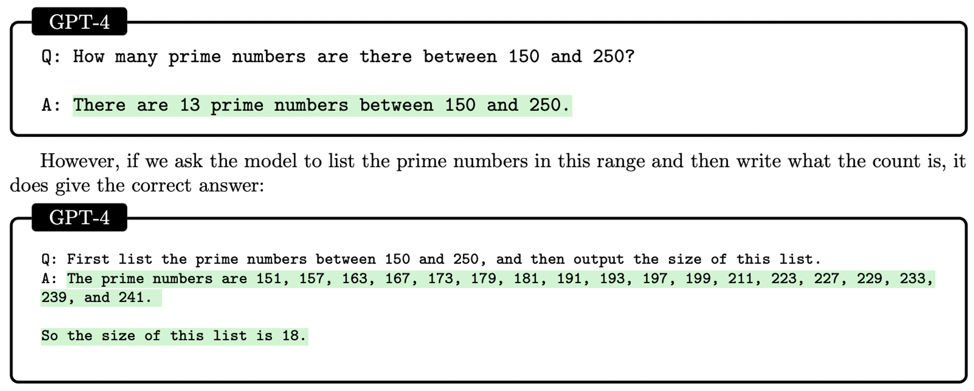
It is actually quite process-consistent. Here, it was asked to prove that primes are infinite. In the proof, it started with prime P, and then added a prime Q as part of its proof. Why did it pick the letter Q? If you start with a different letter than P, or if you tell it something about its alphabet, then it does correctly increment the letter based on the new alphabet schema. It seems to understand the “process” that led to its picking Q.

It does seem to understand solutions, not just memorize numbers:
If we give it a problem, and then we change the problem’s numbers, GPT-4 still gets it right while older models flounder. That suggests this is more than just rote memorization.

Solving coding problems:
It is very good at solving coding problems. Leet Code is a repository that it couldn’t have memorized during training because it changes all the time. It matches human performance.

Music:
It is not very good at producing coherent music in ABC notation.
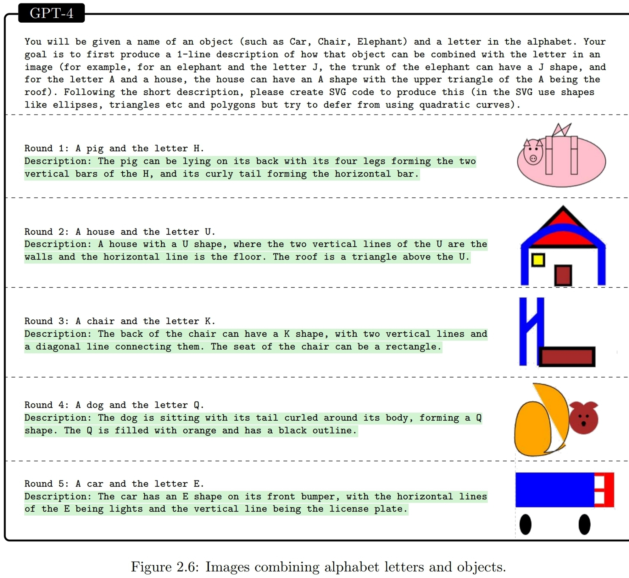
Images:
It understands and can make sense of visual information surprisingly well - even if the information is just encoded in code to create images.
Explaining the Transformer
(Jan 2023, link)
Here is how a transformer works:
The key idea is that you need to give the neural network the chance to combine any two tokens of an input sequence - no matter where those tokens are in the input text. If you just give it a series of input tokens and some window, it will never be able to combine what it first read with what it’s currently reading. So we’re going to create a cross-product of all input tokens as an input to the network.
You have an input sequence of 5 tokens, for example “I like my input sequence”. Input = [“I”, “like”, “my”, “input”, “sequence”]. This is a tensor of dimension 1x5.
Calculate the embedding vector for each token. An embedding vector will turn each token into a vector of a larger dimension, say, a vector with 16 components. So the input sequence now becomes a tensor of dimension 16x5. (Each token goes from being a scalar of dimension 1 to being a vector of dimension 16.)
Now you take three matrices:
The query matrix Wq
The key matrix Wk
The value matrix Wv
You’re going to multiply each embedded token vector with each of these. So we know that each of these matrices has to have width 16. We can pick the height of each matrix freely. So each matrix turns a 16-component token vector into a vector of another dimension, and that’s really it. There is still just one independent vector for each token at the end of this.
The only additional constraint is that matrices Wq and Wk need to have the same height, because of what we’re going to do next. But for now, let’s pick the following:
Query matrix Wq is a (24, 16) matrix
Key matrix Wk is a (24, 16) matrix
Value matrix Wv is a (28, 16) matrix
Let’s do one example calculation step: take the second token from the input sequence, x[2]. That was “like” in the input sequence, and became a 16-dimensional vector x[2].
Multiply Wq * x[2] => q[2] which is a 24-dimensional vector
Multiply Wk * x[2] => k[2] which is a 24-dimensional vector as well
Multiply Wv * x[2] => v[2] which is a 28-dimensional vector
After doing this (independently) for all tokens in the input sequence, you went from having 5 16-dimensional vectors to having 3 times 5 vectors (3 vectors for each input token), of which 5 vectors have dimension 24 (the q[i]), another 5 vectors have dimension 24 (the k[i]), and 5 vectors have dimension 28 (the v[i]).
Now we’re getting to the cross-attention! So far, none of these steps combined any of the input tokens - we still have completely independent vectors for each input token (only more than one now for each token).
Now, create the full cross-product of the query and the key vectors, so:
w[i,j] = q[i] * k[j]
This works because we forced all q[i] vectors (of which there are 5, one for each input token) to have the same dimension as all k[i] vectors (of which there are also 5)
You could have just multiplied the original embedding vectors, but by first multiplying it with two matrices Wq and Wk, we’re giving the network more parameters to tune
Note the dimensionality of w[i,j]: it’s a (5, 5) matrix! It has the same dimensionality in width and height as the length of the input sequence. Any of the “intermediate” dimensionalities from above (whether it’s the 16 dimensions of the embedding space, or the dimensions of the matrices), disappeared.
Now, we’re going to calculate the actual normalized attention weights. If you think about w[i,j], you can interpret it as weights already: for example, w[2,j] is a vector of dimension 5, because it has a “weight” for how much each of the input tokens should “influence” token 2. For each token, you have a completely independent set of weights for each other token.
Really, this final matrix w[i,j] is what you were after all along - but it’s just easier to break it down into two intermediate matrices Wq and Wk, which you multiply to get the final matrix.
If we really want “weights” that weigh each of the 5 input tokens for, say, token 2, then we need those 5 weights to sum up to 1 and all be in the range [0, 1]. Then we can interpret them as “probabilities”. We do that by using the softmax function on each weight vector w[i,j].
The softmax function is simple: you can give it a list of 5 input values which can be anything, say x(i) = [-5, 100, 3, -10, 0]. It will take the exponential of each number, then divide by the sum of that. So y(i) = [exp(-5), exp(100), exp(3), exp(-10), exp(0)] / (exp(5) + exp(100) + exp(3) + exp(-10) + exp(0)). It knows how to deal with negative numbers, and it forces everything into [0,1] and to add up to 1.
So now we have the matrix a[i,j], and each row vector a[i] has five elements which are in the range [0,1] and add up to 1. So vector a[2] = a[2,j] with j=1..5 has the 5 weights that get multiplied with each of the 5 input tokens to get their “weighting” as they relate to input token 2.
Finally, we calculate the actual vector that gets fed into the neural network. That’s what the “value” matrix from above was for: it effectively just “passes through” each original token. Remember, each token in embedding space is a 16-dimensional vector, and multiplying it with Wv turned it into a 28-dimensional vector (where the 28 is really arbitrary).
However, also remember that a[i,j] is a 5x5 matrix. Where is the dimension 28? It’s nowhere in here. Instead, each token weight is just a scale up/down factor for the 28-dimensional vector that represents an input token.
Let’s say that the attention weight vector for token 2 (which was x[2]) is a[2,j] = [0.2, 0.3, 0.1, 0.2, 0.2]. We also have five value vectors v[j] = Wv * x[j]. Each of these value vectors has dimension 28. The simple calculation here is now z[2] = a[2,1] * v[1] + a[2,2] * v[2] + a[2,3] * v[3] + a[2,4] * v[4] + a[2,5] * v[5]. Each of these a[] elements is just one number (a weight), and we know that they sum up to 1 because we normalized them with softmax.
So you’re really just weighting the 5 28-dimensional input vectors to get one final 28-dimensional vector z[2]. Again, the dimension 28 is arbitrary, we can pick that by picking the value matrix Wv.
One final modification: right now, we have one matrix each for Wq, Wk, Wv. Instead of one set, we could have multiple sets of these three matrices. They could all get calculated independently. That would give us several z vectors at the end, not just one of them. Each is then called an “attention head”, and this is what is meant with “multi-head attention”.
This is a nice image that sums it all up:

As a final modification, instead of just using the input sequence, we can also mix the input and output sequence. Nothing else changes - the input sequence vector just gets longer.

Python Code Implementing a Transformer
This is a great step-by-step transformer implementation in Python.
An Overview On Language Models: Recent Developments And Outlook (Mar 2023)
(link)
Really just an overview of a bunch of natural language processing models, including LLMs.
Harnessing the Power of LLMs in Practice: A Survey on ChatGPT and Beyond (Apr 2023, added 5/7/23)
This is a survey paper summarizing various insights on LLMs. Mostly already covered elsewhere, but below is a helpful flowchart on how to decide on fine-tuning vs. few-shot LLMs:

Also interesting insights on tasks where performance in larger LLMs gets worse:
On certain tasks, with the size of LLMs increasing, the performance begins to decrease, such as Redefine-math: tests whether language models are able to work with common symbols when they are redefined to mean something else; Into-the-unknown: requires the model to choose which piece of information would help answer a question; Memo-trap: asks an LM to write a phrase in a way that starts like a famous quote but ends differently. This is also called Inverse Scaling Phenomenon.
Another interesting phenomenon observed in the scaling of LLMs is called the U-shaped Phenomenon. As the name implies, This phenomenon refers to that as LLM size increases, their performance on certain tasks initially improves but then starts to decline before eventually improving again, such as on: Hindsight-neglect: it tests whether language models are able to assess whether a bet was worth taking based on its expected value; NegationQA: this task takes an existing multiple-choice dataset and negates a part of each question to see if language models are sensitive to negation; Quote-repetition: it asks models to repeat back sentences given in the prompt, with few-shot examples to help it recognize the task.
For emergent abilities, one explanation is that there may be multiple key steps for a task and the LLM cannot handle this task until it’s large enough to handle every step. But we don’t really know yet.
Do Machine Learning Models Memorize or Generalize?
(Aug 2023, link)
An awesome paper from Google Research on grokking: when do machine learning models simply mimic their training data, and when do they actually understand what they’re doing? Here is a fantastic chart that shows the difference: initially, the model just gets extremely good at memorizing its training data - but eventually, after more training, accuracy on test data suddenly improves a lot. That’s when the model figured out how to generalize.

The paper starts with training a model for a very simple task: given a random sequence of 30 0s and 1s, predict if there is an odd number of 1s in the first three digits. A generalizing model should only use the first three digits of the sequence; if the model is memorizing the training data, it will also use the subsequent distracting digits. The model is a 1-layer perceptron, i.e., all neurons in that one layer are fully connected to the input. The training initially just memorizes the training data, and only eventually the model generalizes.

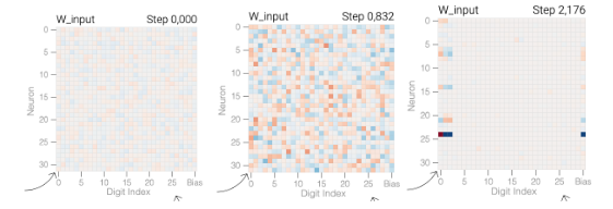
Here are the neuron weights during the training: at left, before it gets going; in the middle, when it memorized the training data; at right, when it generalized. We can see that when it just memorizes training data, it uses all inputs in all neurons - it can reproduce the data, but it hasn’t figured out what it’s doing. When it is generalized, it has figured out that it only needs the first three digit inputs.
What is super interesting is that we can see directly why this transition occurs: it is because of the dual training objectives we have. One objective is to output a high probability for the correct label (called minimizing loss): i.e., replicate the training data. But the other is to have weights with low magnitudes (called weight decay): i.e., make the weights simpler.

What is remarkable is the dynamics of the training: in the chart above, it looks as if the model suddenly generalizes - test loss drops off suddenly (at training step 2,128). But in fact, if we look at all the weights in the chart below, they all start shrinking around step 1,200 and just keep going down. The rapid generalization occurs when the last weights connected to the distracting digits are pruned by weight decay.

You need to tune the training hyperparameters just right to achieve grokking. With too little weight decay, the model can’t escape overfitting the training data.8 Adding more weight decay pushes the model to generalize after memorizing. Increasing weight decay even more causes test and train loss to fall together; the model goes straight to generalizing. And with too much weight decay the model will fail to learn anything.
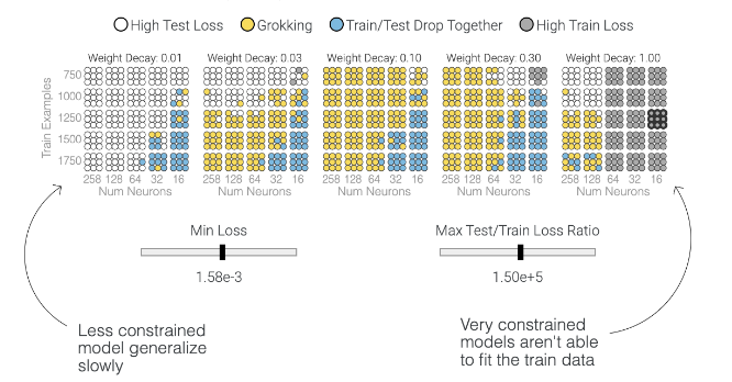
The paper then shows how models fail to grok, depending on model size, weight decay and hyperparameters. Below, each circle is a model with particular characteristics. Only for some of them does the model achieve grokking.
The paper then looks at another model which calculates a + b mod 67. They show that for this task, the model needs to figure out how to extract periodicity from the numbers. It does so successfully.
Thinking Like Transformers
(Jul 2021, link)
Transformers have a very explicit structure: a sequence of N input tokens goes into an attention layer, the attention layer applies key-query-value transformations and produces N output tokens, those N tokens go into a feed-forward layer, which then produces another N final tokens. That repeats throughout all the transformer layers. So absolutely every layer of the transformer looks like this:
The idea behind this paper is simple: this means transformers - without any pretraining whatsoever, simply starting from this structure - can “implement” some very specific types of programs.
Without having any idea how training works, or what we’re training towards, there are very specific variables flowing between each of these layers, and we can simply try to capture what those signals do in a high-level programming language.
That is what RASP is: it provides a very limited instruction set in Python that exactly mimics what is happening in these transformer layers. That should let us specify the smallest possible “programs” that a transformer can implement. (Whether a virgin transformer would then learn exactly that program is a totally different question - but in trying to implement a particular program, we might learn that it’s simply not possible using RASP, which then means that the transformer should have no ability to figure it out either.)
We have three layers:
The input layer. Here we put in the input sequence.
The feed forward layer. Here we can apply a transformation to each token - but independently. We can’t just do something that requires two or three tokens, because it’s not how the feed-forward network would do it either. Each token for itself.
The attention layer. Here we can write down a matrix that mixes tokens together, before we present them to the next layer. So after the token-only feed forward layer, this is our mixing-token layer.
Here is how each layer works. Starting with the input layer. We only have two commands here.
tokens.input([5, 2, 4, 5, 2, 2])This will set the input token sequence to those numbers. And:
indicesThis will always simply return the index list [0,1,2,3,4,5].
Now the feed forward network. This lets us specify any operation on the token input sequence - but applied independently to all tokens. For example:
tokens == "l"This us [0,0,1,1,0] if you for input = [h,e,l,l,o]: 1 wherever we have the letter l, and 0 elsewhere.
model = tokens * 2 - 1model.input([1, 2, 3, 5, 2])This gives us [1,3,5,9,3] for the input [1,2,3,5,2]: double each token and subtract 1. We can also use the indices sequence here:
model = tokens - 5 + indicesThis gives us [-4,-2,0,3,1] = [1-5+0,2-5+1,3-5+2,5-5+3,2-5+4] for the input [1,2,3,5,2]. Again, this is all element-wise manipulation, you can’t mix two tokens together to do anything.
They offer a slightly more complicated construct here: where is a sort of if-statement.
where((tokens == "h") | (tokens == "l"), tokens, "q")This yields [h,q,l,l,q] for input [h,e,l,l,o]: if the input token is h or l, replace it with q, if not then just repeat the input token.
Finally you can define your own functions to apply here:
squared = tokens.map(lambda x: x^2)
This yields [0,1,4,9,16] for the input [0,1,2,3,4]. Here we have to be careful, because this has to all fit into one feed forward network, and if we make the function to complicated it wouldn’t fit in there. But at least in theory this is all possible.
Finally, the attention layer. That’s where tokens can get mixed together. This works because attention layers let us define square matrices that can combine any token with any other token. They call these matrices “selectors”. This is straightforward once you wrap your head around it. You can think of these selectors as squares with three inputs: the key from the top, the query from the left, and the value from the bottom. Your actual selector derives from comparing the key with the query sequence. And your value sequence then gets multiplied with that resulting matrix (the selector). So let’s say we define this selector, and pass the sequence (1,1,1,1,1) into it:
(key(tokens) == query(tokens)).value(1)This means that our selector is 1 in each place where the input token is equal to the output token. But note that this is really just pairwise comparison, so both “l” work. Where the two are equal, you get 1, elsewhere 0. Then we just multiply each row with the value sequence, and we add up the number of 1s we get in each row. That’s the output: (1,1,2,2,1).
That’s it: the keys are coming from the top, the queries are coming from the left, and those two get combined into an attention matrix; then you multiply that matrix with the value vector, and you add up those numbers across the rows.
You can use the RASP language here. The great thing about this Colab notebook is that it produces the graphical illustrations entirely based on the code you put in! Here is a summary of the language:
query(1) => produces a query (column) vector of just 1s
key(2) => produces a key (row) vector of just 2s
Naming functions: you can name a function that you can then re-use. Below we show that for cumsum(). You always need to use function().input() to run sequences through it.
In building selectors, you need to always combine keys and queries, the language won’t understand anything else. For example, if you want to select just the first 5 elements of a sequence, then you can’t just say key(indices) < 5. Instead, you need to say key(indices) < query(5). So you create a query vector of 5s and can then compare that to the key vector.
You can go back and forth between sequences and selectors. For example, you might create a sequence from sub-selecting some part of the input sequence, then use that to build a selector, then apply that selector to the entire input sequence. That’s all allowed: you don’t need to have the same input sequence flow through the entire logic.
Let’s do a full custom example. The goal here: you get an input sequence of 10 tokens. The right-most 5 tokens are a selection mask and get applied to the left-most 5 tokens. For example, the string “h e l l o 0 1 0 1 1” should yield “0 e 0 l o 0 1 0 1 1”: we use the 1s at the right to select the letters at the left.
How we do this conceptually:
We need a diagonal matrix that has the second part of the string (0 1 0 1 1) as a diagonal matrix applied to the first half of the string. Then, if we multiply the entire string with that matrix, we’ll get the correct letters selected.
So we have to first create a string that has the second part of the string (0 1 0 1 1) repeated twice, also in the first part of the string. So we need (0 1 0 1 1 0 1 0 1 1).
We get that by creating a 10x10 matrix that has a diagonal matrix in the 5 bottom-right elements, but also in the 5 top-right elements. If you think about the original input string coming in from the bottom, it means that off to the right you get the correct output string.
This is how the first phase will work:
Now that we have a string that repeats the mask sequence twice, we can turn that string back into a selector. This is a crucial capability: we can use one output sequence to create another selector. Because, again: this doesn’t give us a selector, this gives us an output sequence (0 1 0 1 1 0 1 0 1 1).
Now we turn that sequence into a selector that’s just a diagonal matrix repeating those numbers.
Then we multiply the original input sequence with that final diagonal mask matrix.
Here is how this looks in terms of output from RASP:
First, copy the mask sequence into the whole string. The intermediate sequence is at the right.
Second, we use that sequence to create another selector. See the sequence at the top (the key), getting compared to the left (the query). We get the diagonal mask matrix. Then we send in the original sequence as value from below, and we get the output at the right, correctly masked.
What Algorithms Can Transformers Learn? A Study In Length Generalization
(Oct 2023, link)
A very foundational question for transformers is: when do they generalize, and when do they parrot? Meaning, when you feed them enough solutions to a particular problem, do they actually figure out how to solve that problem generically and for any input variation, or do they simply memorize training data? This paper makes it clearer when transformers are able to do the former: to find generalized solutions.
(There is actually a “third way” in between finding general solutions and mimicing training data: the “Faith and Fate: Limits of Transformers on Compositionality” paper (link) showed that in doing long-form addition, transformers memorize and then re-compose small-number additions. For example, if you memorize 3 + 3 = 6, you can actually also solve 33 + 33 = 66.)
Here is this paper’s very foundational insight: if you can take a problem and write a “RASP-L program” to solve it, then you should be able to get a transformer to find a general solution for it. If such a program doesn’t exist, then a transformer won’t be able to find a general solution. This is a really powerful, foundational insight, because it rules out a class of problems from ever having a transformer finding a general solution. See the chart below: the counting task (get a transformer to count upwards) does have a RASP-L program. So if you train a transformer with examples of up to length 10, then the chart at the right shows that you get generalized solutions that work up to length 20 pretty well. Training to length 40 works pretty well up to length 60, and so on. But the “parity” problem does not have a RASP-L program, so transformers have no chance whatsoever to go even length += 10 over the training data. This is a cool insight.
(Another paper, A Logic For Expressing Log-Precision Transformers (link), takes a somewhat similar approach that should somehow get connected to this: it proves that transformers are capable of implementing first-order logic expressions with majority-vote classifiers. That also allows a very specific family of expressions to be implemented and rules out others. That should be connectable to the results in this paper.)
RASP-L is a very particular programming language that simply models the kinds of data transformations you can do in the transformer architecture. It has a really simple intuition: there are only two kinds of transformations that the transformer architecture allows.
Element-wise transformation of a sequence: for example, if the transformer’s input sequence is [0, 1, 2, 1, 3], then the element-wise operation x^2 would yield [0, 1, 4, 1, 9].
Attention-selection transformation of a sequence: this lets us build any kind of attention matrix using any kind of input sequence. For that, we can use two input sequences: a “key” and a “query” sequence. The attention matrix then gets defined as comparing those two sequences across all of their elements. For example, if the “key” sequence is [1, 2, 4] and the “query” sequence is [2, 1, 3], then we can build an attention matrix by saying key <= query and we get: [[1,1,1], [1,0,1],[0,0,0]]. We get this by simply going through all elements in the “key” sequence and comparing the element vs. each element in the “query” sequence and checking if it’s smaller or equal.
After that, we can multiply that attention matrix with an input sequence to get another sequence.
That’s it! We can then layer as many of these as we want. So we could take an input sequence, transform it element-wise, then use that and the original sequence to build an attention matrix, then multiply that matrix with the input sequence. Then use that to build another attention matrix, and so on. Eventually we get an output sequence.
The paper’s basic insight: the “RASP-Generalization Conjecture”. Which states: a decoder-only autoregressive Transformer is likely to length-generalize when trained to completion on an algorithmic task if the following conditions hold.
1. Realizability. The true next-token function for the task can be represented by a single causal
Transformer which works on all input lengths.
2. Simplicity. This representation is “simple”, meaning it can be written in RASP-L (a learnable
subset of RASP).
3. Diversity. The training data is sufficiently diverse, such that there does not exist any shorter
RASP-L program which agrees with the task in-distribution but not out-of-distribution.
Remarkably, the above features are empirically correlated with: (1) generalization to longer lengths out-of-distribution, and (2) faster train optimization in-distribution.
This means: if you can write a RASP-L program, then it’s likely that you can train a transformer with less length in your training examples, and it will still figure out the general algorithm to solve your problem.
Important: the realizability condition seems very strong (you need one transformer to work for all input lengths). But it turns out that considering representability in the unbounded length setting is a good heuristic for learnability in bounded length settings. Intuitively, if a task requires a different Transformer for each input length, then it may be an “unnatural” task for Transformers, and unlikely to generalize well.
Note: the language defined in this paper, RASP-L, is both easier and more constrained than the RASP in the original paper. It provides a bunch of helper functions (like index_select which sub-selects a number of indexes from a sequence) which are easy to transformers to implement. It also forces the language to be “causal” which means you can only combine forward-looking keys with queries.